Getting Started with StatsBomb Open Data in Python (statsbombpy)
From pip install to your first leaderboard, in real Python.
StatsBomb publishes a genuinely free, genuinely rich open dataset — 80 competition-seasons covering 24 distinct competitions, including the full 2022 World Cup — and all it takes to unlock it is a single Python package and about fifty lines of code. No account. No API key. No scraping. Here is exactly how to get from nothing to a top-xG leaderboard, with every command copy-pasteable.
Installation
Two libraries carry the load: statsbombpy, StatsBomb's official Python client, and pandas for the usual wrangling. Add matplotlib if you want charts (you do).
pip install statsbombpy matplotlib pandasThat is the entire setup. The package talks directly to StatsBomb's public GitHub-hosted JSON files, so nothing lives on your machine until you ask for it. One import and you're ready.
from statsbombpy import sbThe data model: competitions → matches → events
StatsBomb organises everything in three layers, and understanding them upfront saves a lot of confused index errors.
Competitions. The outermost layer. Calling sb.competitions() returns a DataFrame with one row per competition-season — the 2022 World Cup is one row, the 2018 World Cup is another. As of this writing the free tier has 80 such rows across 24 distinct competition names.
Matches. Once you have a competition-season you can call sb.matches(competition_id=..., season_id=...) to get all matches in that tournament. The 2022 World Cup returns 64 rows, one per match, each carrying kick-off time, final score, home and away team names, and a match_id you'll use for the next step.
Events. The real payload. sb.events(match_id=...) returns every on-ball action in a single match: passes, shots, carries, duels, goalkeeper actions, set pieces. A match might produce a few thousand rows. Each event has a type, a team, a player, a location, a timestamp, and a cluster of type-specific columns — pass_end_location for passes, shot_statsbomb_xg for shots, and so on.
Loading competitions, then drilling down
The competition call is the starting point for almost every analysis. It is free and fast — it just fetches a small JSON file.
from statsbombpy import sb

# 1 — what's available? competitions() returns one row per competition-season.
comps = sb.competitions()
print(f"{len(comps)} competition-seasons available, "
      f"{comps.competition_name.nunique()} distinct competitions.")
Running this against the current open dataset prints 80 competition-seasons available, 24 distinct competitions. That range includes Champions League campaigns, La Liga seasons, the Women's World Cup, NWSL, and the full men's World Cup from 2018 and 2022. The 2022 tournament is competition_id 43.
# 2 — pick a competition-season (men's 2022 World Cup) and list its matches.
season = comps[(comps.competition_id == 43) & (comps.season_name == "2022")].iloc[0]
matches = sb.matches(competition_id=43, season_id=int(season.season_id))
print(f"{len(matches)} matches at the 2022 World Cup.")
That prints 64 matches at the 2022 World Cup. — every group stage game through the final. Each row contains both team names, the final score, and the match_id needed for the next step.
Pulling shots across a whole tournament
Calling sb.events() once per match and concatenating the results is the standard pattern for tournament-level analysis. It takes a minute or two on a normal connection — each match is a separate HTTP request — but it is straightforward:
# 3 — pull events for every match and keep the shots.
shots = []
for match_id in matches.match_id:
    ev = sb.events(match_id=int(match_id))
    shots.append(ev[ev.type == "Shot"])
shots = pd.concat(shots, ignore_index=True)
shots["xg"] = shots.shot_statsbomb_xg.astype(float)
The explicit astype(float) is worth explaining: shot_statsbomb_xg comes back as a mixed-type column because StatsBomb stores non-shot events in the same DataFrame with nulls in shot-specific columns. Casting it after filtering to shots only avoids the occasional coercion warning downstream.
From here, building the leaderboard is one line of pandas groupby:
# 4 — the ten players with the most expected goals.
top = shots.groupby("player").xg.sum().sort_values(ascending=False).head(10).round(2)
goals = shots[shots.shot_outcome == "Goal"].groupby("player").size()
The goals Series counts actual goals for the same players, which is what makes the output interesting: comparing xG to actual goals tells you immediately who was clinical and who left chances on the pitch.
Building the chart
The companion script produces a horizontal bar chart, which works better than a vertical one here because the player names are long. The top three bars get an accent colour to pull the eye; the rest are the house green. The label on each bar prints both xG and actual goals so readers don't have to cross-reference a table.
import matplotlib.pyplot as plt

PAPER, GREEN, GREEN_DK, ACCENT, INK = "#fbfaf3", "#0a5a3f", "#073e2c", "#f4c20d", "#16231c"

fig, ax = plt.subplots(figsize=(8.8, 5.6))
names = list(top.index)[::-1]   # reverse so highest is at the top
vals  = list(top.values)[::-1]
colors = [ACCENT if v >= sorted(vals)[-3] else GREEN for v in vals]

ax.barh(names, vals, color=colors, edgecolor=GREEN_DK, linewidth=0.5)
for i, (n, v) in enumerate(zip(names, vals)):
    ax.text(v, i, f"  {v:.1f} xG ({int(goals.get(n, 0))}G)",
            va="center", fontsize=9, color=INK)

ax.set_xlabel("Total expected goals (xG)")
ax.set_title("Most xG at the 2022 World Cup", loc="left",
             color=GREEN_DK, fontweight="bold")
ax.spines[["top", "right"]].set_visible(False)
ax.margins(x=0.18)
fig.patch.set_facecolor(PAPER)
ax.set_facecolor(PAPER)
fig.savefig("statsbomb-top-xg-wc2022.png", dpi=150,
            bbox_inches="tight", facecolor=PAPER)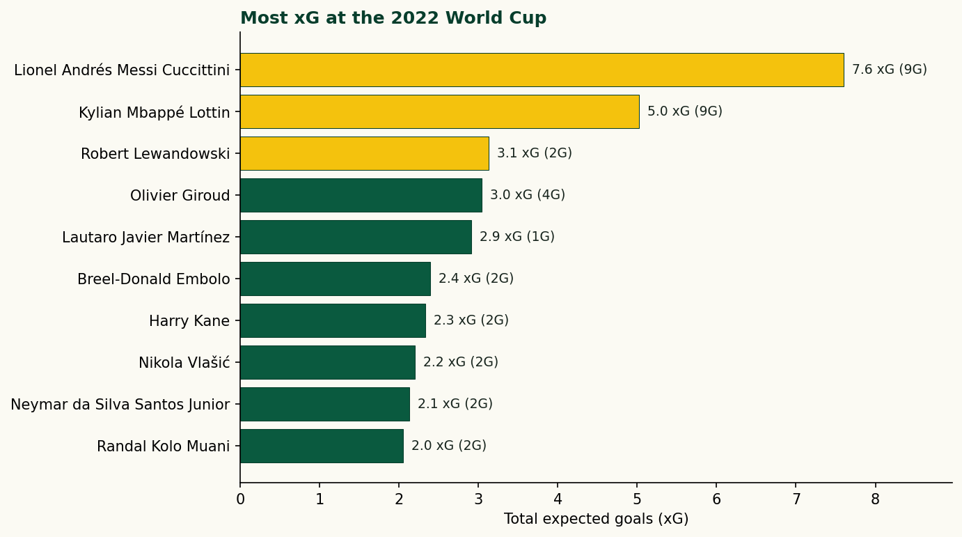
Reading the leaderboard
The numbers tell a vivid story. Here is the full top ten, drawn directly from the data:
| Player | xG | Goals |
|---|---|---|
| Lionel Andrés Messi Cuccittini | 7.60 | 9 |
| Kylian Mbappé Lottin | 5.02 | 9 |
| Robert Lewandowski | 3.13 | 2 |
| Olivier Giroud | 3.04 | 4 |
| Lautaro Javier Martínez | 2.91 | 1 |
| Breel-Donald Embolo | 2.39 | 2 |
| Harry Kane | 2.33 | 2 |
| Nikola Vlašić | 2.20 | 2 |
| Neymar da Silva Santos Junior | 2.13 | 2 |
| Randal Kolo Muani | 2.05 | 2 |
Messi led the tournament with 7.60 xG and converted 9 goals — heavily outperforming his model, much of it through penalties. Mbappé matched that goal tally from only 5.02 xG, a finishing rate that speaks for itself. Lewandowski sits third on 3.13 xG but scored only 2 goals: Poland's group-stage exit meant he never converted the chances he found. Lautaro Martínez is the most striking entry — 2.91 xG, 1 goal, the clearest case of a striker who was in the right places and made nothing of it.
Attribution — don't skip this
StatsBomb's open data comes with a use requirement. Any public work that uses it — a blog post, a tweet, a dashboard — must carry clear credit to StatsBomb. The exact wording they request is "Data provided by StatsBomb" or "Powered by StatsBomb", plus a link to statsbomb.com. The data is free; the attribution is the price. It is a fair deal and worth honouring.
If you are building something that will be published — even informally — add a small text label to every figure and a note in any accompanying write-up. The companion script already appends Data: StatsBomb open data to each chart's source line; replicate that pattern and you're covered.
Where to go next
Once you are comfortable pulling shots you are a short step from most of the standard analyses in football analytics:
- Filter events to
type == "Pass"and uselocationandpass_end_locationto draw a pass map — the mplsoccer tutorial on this site covers that exactly. - Group events by
periodto study how a team's pressing intensity changes as a match ages. - Pull the full
freeze_framecolumn from shot events to see where the defence was standing at the moment of each shot — StatsBomb's data is one of the few free sources with that level of detail. - Loop over every competition-season available, not just the World Cup, to build career-level xG totals for any player who appears in the open data.
The full companion script is at scripts/getting-started-with-statsbomb-open-data.py in this site's repository. Change the competition_id filter and it maps any of the 24 competitions StatsBomb has opened up.
Sources & further reading
- Free textbook: Chapter 4: Python Tools for Soccer Analytics — the theory behind this, at DataField.dev.
- statsbombpy on GitHub — the official Python client, installation notes, and changelog.
- StatsBomb open data — the raw JSON files; also where you find the spec documents describing every column.
- StatsBomb — the company behind the data; required attribution destination for any published work.
- mplsoccer documentation — the plotting library that turns StatsBomb coordinates into pitch visualisations.
- pandas documentation — the wrangling layer used throughout the companion script.