Do Football Goals Follow a Poisson? Testing the Standard Model on All 64 Games of 2022

If you have ever seen a model spit out "Argentina 38% to win, 31% draw, 31% Brazil," you have seen the Poisson distribution at work. It is the quiet engine under almost every scoreline forecast in football: assume each side scores goals like raindrops hitting a windowpane — rare, independent events arriving at some steady rate — and the whole grammar of match odds falls out of one little formula. The model is everywhere. What I rarely see anyone do is the obvious next step: take real results and ask whether goals actually behave that way. So I did, with all 64 matches of the 2022 World Cup, and the answer is the interesting kind of "almost."

The model, in one line

The Poisson distribution gives the probability of seeing exactly k goals when the average rate is λ (lambda):

Poisson probability of k goalsP(k) = λ^k · e^−λ / k!

That's it. Feed it a rate and it hands back the full distribution of outcomes. The appeal for football is that it needs only one number per team — an expected goals rate — and the assumptions sound exactly like a low-scoring sport: goals are rare, they don't (the theory says) depend on each other, and they fall at a roughly constant rate across the 90 minutes. Set λ to the average and you have a parameter-free prediction you can check against reality.

Fitting it to 2022

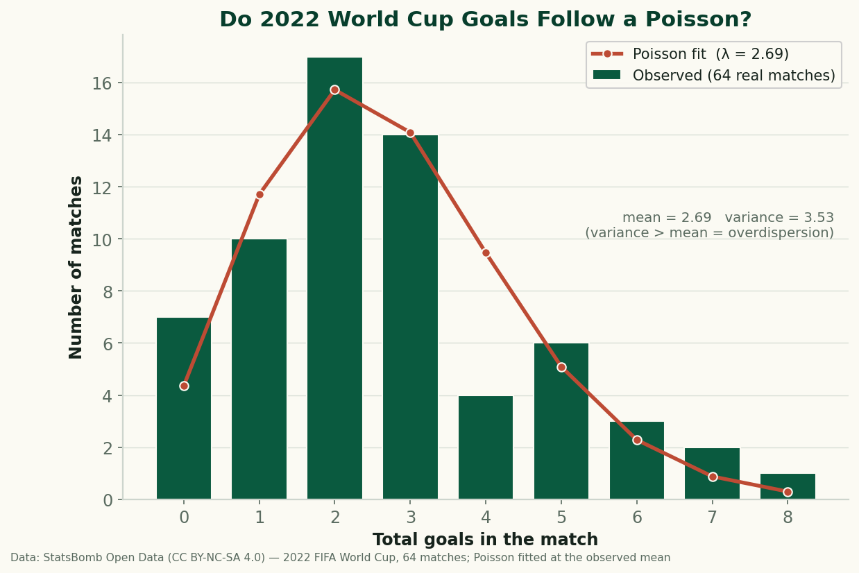
The honest test is simple. Across all 64 matches the 2022 World Cup produced 172 goals, a mean of 2.69 goals per match (add every home_score and away_score, divide by 64 — no model in that step). Set λ = 2.69, compute the Poisson probability of a 0-goal game, a 1-goal game, and so on, multiply each by 64, and you get how many matches of each total the model expects. Lay that next to what actually happened.

A bar-and-line chart comparing the observed distribution of total goals per match at the 2022 World Cup against a fitted Poisson distribution. Green bars show the 64 real matches by total goals; an orange line with markers shows the Poisson expectation at lambda 2.69. The bars are higher than the line at zero goals and in the high-scoring tail, and lower than the line around four goals. A note reads mean 2.69, variance 3.53, overdispersion. — Observed total goals per match across all 64 games of the 2022 World Cup (green bars) versus a Poisson distribution fitted at the observed mean of 2.69 (orange line). The fit is good in the middle and misses at the extremes. Data: StatsBomb Open Data (CC BY-NC-SA 4.0) — 64 matches; Poisson fitted at the observed mean.

Goals in match	Observed matches	Poisson expects
0	7	4.4
1	10	11.7
2	17	15.7
3	14	14.1
4	4	9.5
5	6	5.1
6	3	2.3
7+	3	1.2

Observed counts from StatsBomb Open Data, 2022 FIFA World Cup; expected counts = 64 × Poisson(λ = 2.69).

Look at the middle of that table and the model is genuinely good. Two-goal games: 17 observed, 15.7 predicted. Three-goal games: 14 observed, 14.1 predicted. The single most common scoreline band and the overall right-skewed shape — most games clustering at two or three, a long thin tail of high-scoring ones — come straight out of the formula. For a one-parameter model that knows nothing about who was playing, that is a real success, and it is why the Poisson has survived as the default since Michael Maher formalized it for football in 1982.

Where it breaks — and it breaks in a revealing way

Now read the extremes. There were 7 goalless or near-goalless games where the model expected about 4.4. There were 3 matches of seven or more goals where it expected barely 1. And right in the middle of the upper range, four-goal games, reality came in under the model — 4 observed against 9.5 expected. The pattern is unmistakable: too many blanks, too many blowouts, not enough of the tidy mid-range games the Poisson loves. The distribution has fatter tails than pure randomness allows.

There's a precise name for this. A Poisson distribution has a defining property: its variance must equal its mean. Here the mean is 2.69 but the variance of match totals is 3.53 — a variance-to-mean ratio of 1.31. The real goals are overdispersed: more spread out than the model permits. That single number, 1.31 instead of 1.00, is the whole failure quantified.

Why goals are overdispersed (the part worth keeping)

Two of the Poisson's assumptions are wrong in football, and each pushes the variance up.

First, λ is not the same in every match. I fit one rate, 2.69, to all 64 games — but Spain–Costa Rica is not Croatia–Morocco. A lopsided fixture has a high expected rate and tends to produce a rout; two cagey, well-matched defenses have a low rate and grind to 0–0. When you average genuinely different rates into one number, the result is mathematically guaranteed to be overdispersed: a mixture of Poissons always has variance greater than its mean. The extra blanks and the extra blowouts aren't noise — they're the fingerprints of team quality the single-λ model deliberately ignored. (It's the same heterogeneity that makes a tournament's 64 results spread the way they do.)

Second, goals within a match aren't independent. The Poisson assumes the next goal is as likely after a 3–0 as after a 0–0. Football doesn't work like that: a team three up empties the bench and protects the lead, while a team chasing the game throws numbers forward and either rescues it or gets picked off on the break. Game state couples the goals together, thickening both tails — the comfortable winner adds a fourth and fifth, or the cagey pair never breaks the seal.

How the pros patch it

Nobody who builds these models for a living uses a single league-wide λ. The standard upgrade is to give each team its own attack and defence strength, so every fixture gets its own pair of rates — which is exactly what a real scoreline model does, and what cures most of the heterogeneity problem. On top of that, the Dixon–Coles model (1997) adds a small correction specifically to the low-score cells (0–0, 1–0, 0–1, 1–1) to fix the dependence the plain Poisson gets wrong. The fact that the famous fix targets exactly the low scores is no coincidence — it's the same overdispersion at the bottom of the table you can see in the chart above.

You can feel the per-team version directly. Drop two expected-goals rates into the model below and it returns the win/draw/loss probabilities and the likeliest scorelines — the same Poisson, but with a rate for each side instead of one for the whole tournament:

Interactive scoreline model — enter each team's expected goals to see the Poisson outcome probabilities.

A quick worked check

If you want to confirm the table by hand, take the goalless case. At λ = 2.69, P(0) = e^−2.69 = 0.068, so over 64 matches the model expects 64 × 0.068 ≈ 4.4 blank games. We saw 7. That gap of nearly three matches — about 60% more shutouts than predicted — is small in raw count and large in meaning: it's the low-scoring, low-λ fixtures that a single average rate can't represent. Run the same arithmetic for k = 2 (P = 0.246, expecting 15.7, observing 17) and the middle of the distribution lands almost exactly. The model is right where the matches are average and wrong where they aren't.

The takeaway

"Are goals random?" has a satisfying answer: mostly, but not quite. The Poisson — the simplest possible model of randomness — reproduces the shape of real World Cup scoring well enough that you understand why the entire field is built on it. But it fails in a specific, honest direction. Real goals are overdispersed, because matches aren't interchangeable and goals aren't independent, and that 1.31 variance ratio is the gap between a clean model and a messy sport. The good forecasters don't throw the Poisson out; they keep its skeleton and add back exactly the two things it pretends away — that teams differ, and that the score so far changes what happens next.

Reproduce it

Every number here comes from one results file and the Poisson formula. Total goals per match is home_score + away_score; λ is their mean; the expected counts are 64 × λ^k e^−λ / k!; the overdispersion is just variance / mean. The observed-versus-fitted chart is regenerated by charts/chart_wc2022_poisson.py against the bundled data_layer/wc2022_matches.json — no network, nothing hand-entered.

Sources & further reading

Free textbook: Chapter 20: Predictive Modeling — the theory behind this, at DataField.dev.
Match results: bundled data_layer/wc2022_matches.json — StatsBomb Open Data (CC BY-NC-SA 4.0), 2022 FIFA World Cup, all 64 matches. Charted by charts/chart_wc2022_poisson.py.
M. J. Maher (1982), "Modelling association football scores" — the foundational Poisson treatment.
M. Dixon & S. Coles (1997), "Modelling association football scores and inefficiencies in the football betting market" — the low-score dependence correction.
Companion: Inside the 2022 World Cup: what all 64 results say — the descriptive look this one stress-tests.
How-to: Build a Poisson goals model in Python — the per-team version, in code.
Background: Expected goals (xG) explained — where each team's λ comes from in practice.